Category Archives: Articles

Öræfajökull, bangunnya sang Giant Volcano di Islandia?
Artikel ini ditulis untuk informasi dan overview singkat bagi wisatawan terutama dari Indonesia yang berkunjung ke Iceland untuk meningkatkan kewaspadaan, karena adanya suatu “anomali” yang terjadi pada Öræfajökull , Southeast (SE) Iceland setelah 290 tahun tertidur pulas.
Bahasan series Geologi Islandia kali ini merupakan sambungan dari blog artikel-artikel tentang Islandia yang saya tulis sebelumnya di supersciences dan majalah FGMI Jendela Geosaintis.
2. https://supersciences.wordpress.com/2016/09/25/geologi-islandia-dan-sumber-energinya-part-1-2/
Lokasi dan geologi
Öræfajökull terletak di daerah Tenggara Iceland, merupakan gunung tertinggi dan terbesar di Iceland (2,119 m) yang merupakan gunung api bertipe stratovolcano. Kaldera gunung api ini tertutup oleh es dari salah satu glacier terbesar di Eropa yaitu Vatnajökull. Ketebalan lapisan esnya sendiri bervariasi berkisar antara 400-700 meter. Ketebalan salju rata-rata di setiap tahunnya sekitar 10 m, dan curah hujan rata-rata di sana sekitar 5.000 mm, melebihi semua daerah lain di Iceland. Diameter gunung ini sekitar 20 km dengan volume kurang lebih 370 km³.

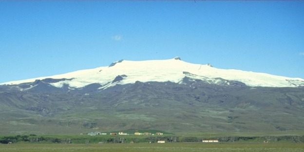
Gambar 1a. Sketsa lokasi
Öræfajökull. Inset disamping menunjukan
lokasi Öræfajökull di Tenggara.
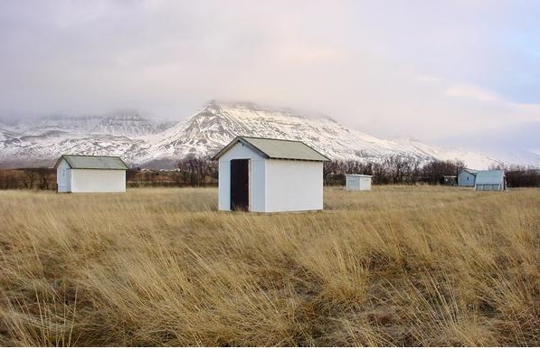
Iceland. Dimodifikasi dari Semellie et al. (2016). Gambar 1b. Foto Öræfajökull dilihat dari arah selatan.
Formasi batuan pada Öræfajökull umumnya berumur kurang dari 0.7 juta tahun dan tipikal Formasi Upper Pleistocene. Volcanic sucessions di daerah ini terbentuk dari lava bantal, hydroclastic tuffs dan breccias, beserta basalt dan lava andesit (Thordarson & Hoskuldsson, 2008). Riolit ditemukan dalam jumlah yang signifikan, baik ekstrusif maupun intrusif hal ini bisa terlihat dari puncak-puncak yang terangkat dari kaldera rim di Öræfajökull adalah sisa-sisa dari kubah lava riolit (Thordarson & Hoskuldsson, 2008).
Sejarah letusan
Öræfajökull dianggap gunung paling aktif kedua di Eropa setelah Gunung Etna di Sisilia, Italia. Dalam masa sejarah tercatat dua letusan terjadi di Öræfajökull, yaitu pada tahun 1362 dan 1727. Sebelum letusan dahsyat di tahun 1362 nama Öræfajökulladalah Knappafell. Nama Öræfi, berasal dari erupsi pertama pada masa bersejarah di daerah dataran alluvial Skeidararsandur di barat dan Breidamerkursandur di timur. Letusan itu hampir menghancurkan kawasan itu dan membunuh sebagian besar penduduk dan ternak mereka. Setelah itu daerah itu tampak seperti padang pasir yang luas, itulah arti kata Öræfi. Puncak riolit Hvannadalshjukur terangkat sekitar 300 m di atas kaldera rim, yang panjangnya sekitar 5 km dan memiliki luas 12 km².
- Erupsi pumice (batu apung) terbesar di Iceland
Beberapa penelitian menganggap erupsi pertama tahun 1362 sebagai erupsi dengan pumice terbesar dan juga erupsi riolitic terbesar di masa sejarah Iceland (Selbekk & Trønnes, 2006; Thordarson & Hoskuldsson, 2008). Magnitude erupsi tahun 1362 ini setara dengan Pinatubo (Filipina) tahun 1991. Volume tephra diperkirakan sekitar 10 km³ (sekitar 2½ km³ riolit kompak) dan menyebar ke arah East-Southeast. Gelombang banjir besar (jökulhlaup) terjadi setelah erupsi, yang kemudian menyapu sebagian besar peternakan di daerah itu. Jökulhlaup terjdi akbat mencairnya glacier, karena interaksi antara magma dan es . Di utara, abu vulkanik jatuh di tanah dan di lepas pantai bagian barat laut, kapal-kapal mengalami kesulitan untuk melewati tumpukan pumice yang mengambang di laut. Deposit pumice yang tebal dapat ditemukan di seluruh wilayah Öræfi saat ini. Tepra Isopach map dan tepra deposit stratigrafi pada erupsi tahun 1362 ditunjukan oleh Gambar 2a dan 2b.
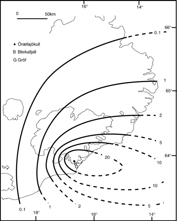
Gambar 2a. Tepra Isopach map erupsi Öræfajökull tahun 1362 (unit dalam cm). Diadaptasi dari Selbekk & Trønnes (2007).

Gambar 2b. Tepra deposit stratigrafi pada erupsi Öræfajökull di tahun 1362, pengukuran di lakukan di daerah Bleikafjall (sekitar 4 km sebelah timur dari crater). Diadaptasi dari Selbekk & Trønnes (2007).
Erupsi kedua terjadi pada bulan Agustus 1727 dan berlangsung hampir setahun sampai April/Mei 1728 (Thordarson & Hoskuldsson). Selama tiga hari pertama dan kolom abu begitu besar, sehingga sulit untuk membedakan antara siang dan malam. Pada erupsi ini tidak banyak korban jiwa dan peternakan yang hancur. Volume tepra yang dihasilkan juga jauh lebih sedikit daripada pada saat erupsi 1362. Jökulhlaup mengarah ke timur melewati Sandfell dan Hof. Tanda-tanda erupsi ini masih terlihat jelas di daerah tersebut sampai sekarang. Setelah 1727 tidak ada aktivitas yang signifikan di Öræfajökull baik seismik ataupun kegempaan sampai pertengahan Summer 2016 (Juni/Juli 2016).
Öræfajökull bangun dari tidur panjang?
- Aktivitas seismik
Sejak pertengahan Summer 2016, aktivitas seismik di Öræfajökull meningkat. Pada bulan Juni dan awal September tahun ini (2017), aktivitas tersebut telah meningkat lebih jauh lagi seperti terlihat pada gambar 3.
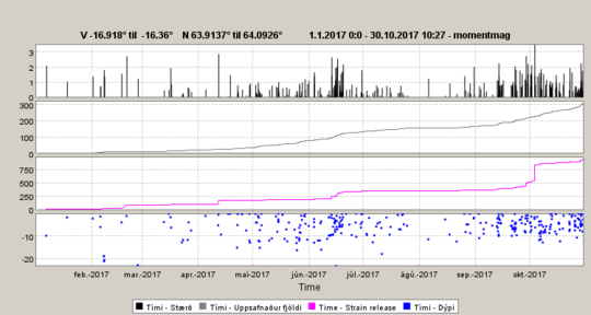
Gambar 3. Seismisitas di Öræfajökull pada tahun 2017: (Paling atas), grafik menunjukkan besarnya gempa yang terdeteksi; grafik berikutnya menunjukkan jumlah kumulatif gempa bumi; Grafik ketiga menunjukkan momen seismik kumulatif. Dari grafik ini terlihat dengan baik gempa M3.5 yang diukur pada awal Oktober 2017. Ini adalah gempa terbesar yang terdeteksi di gunung berapi Öræfajökull sejak awal pengukuran; Grafik terakhir menunjukkan kedalaman gempa di kilometer. (http://en.vedur.is/about-imo/news/new-seismic-stations-installed-around-oraefajokull)
- Terbentuknya Ice Cauldron
Pertengahan November 2017 ini Aerial photo dan citra satelit (Optikal dan Radar) menunjukan adanya ice cauldron yang terbentuk pada lapisan es di Öræfajökull (Gambar 4a,4b,4c). Ice cauldron ini baru terlihat di bulan November 2017 dengan diameter 1 km dan kedalaman 10-20 meter (Iceland Met Ofice).


Gambar 4. Ice cauldron terbentuk pada permukaan es di Öræfajökull terlihat dari (a) pesawat (Foto oleh Ágúst J. Magnússon) ; (b) dan (c) Citra Satelit Landsat 8 dan radar Sentinel 1A yang diproses oleh tim Volcanology dan Natural Hazard Grup, University
Apa itu Ice Cauldron?
Ice cauldron merupakan sebuah depresi di permukaan glacier biasanya terbentuk dengan mencairnya es di bagian dasarnya. lalu apa yang menyebabkan mencairnya permukaan glacier tersebut? Ice cauldron dimungkinkan terjadi akibat adanya aktivitas geotermal di bawah glacier, baik itu hydrothermal upwelling atau magma yang mulai menjalar naik dan terjadi subglacial eruption (Gudmunsson, 2007). Subglacial eruption adalah erupsi yang terjadi dibawah glacier, erupsi tipe ini umum terjadi di Iceland terutama saat Iceland masih berada dalam zaman es yang dimana seluruh daerahnya tertutup oleh glacier.
Berdasarkan bentuk dan ukuran Ice cauldron dapat dibagi menjadi tiga, yaitu:
- Depresi dangkal yang tidak terlihat adanya concentric crevasses. Kedalaman Depresi ini hanya sebagian kecil saja dari ketebalan es total. Di Iceland tipe ini sangat umum di dan biasanya lebar <1 km dan umumnya kedalaman 10-30 m. Biasany cauldron jenis ini terbentuk akibat adanya hydrothermal upwelling dibawah glacier (Gambar 5a dan 5b) (Gudmunsson, 2007).
- Depresi dalam dan berat namun tidak sampai ke dasar gletser. Kedalaman
dari ice cauldron ini bisa menjadi pecahan yang cukup besar dari total ketebalan es. Diameter depresi jenis ini mulai dari seratus meter hingga beberapa kilometer, dengan kedalaman 50-200 m(Gambar 6a dan 6b) (Gudmunsson, 2007). - Depresi sangat dalam dan berat, biasanya didominasi oleh dinding es vertikal dan
sampai ke dasar glacier. Ice cauldron ini biasanya membentuk danau yang dibendung oleh es bagian dasarnya (Gambar 6c) (Gudmunsson, 2007).

Gambar 5. Skema hubungan ice cauldron dan geothermal activity
daerah, (a) air terakumulasi akibat hydrothermal upwelling, (b) air terus mencair akibat hydrothermal upwelling (Diadaptasi dari Gudmusson et al. 2007)

Gambar 6. Skema mencairnya glacier akibat subglacial eruption, (a) membentuk ice cauldron tipe
(1) yang cepat berkembang menjadi tipe (2) (b) magma mulai naik sehingga menjadi ice cauldron tipe (3) (c) danau terbentuk akibat subglacial eruption. (Diadaptasi dari Gudmusson et al. 2007)
Dari skema diatas dan hasil pengamatan terlihat jelas bahwa Öræfajökull sedang berusaha untuk bangun dari tidurnya, apakah akan mencapai ice cauldron tipe 3 (Erupsi) ? apakah akan sama seperti 1362 dengan pyroclastic flow yang benar benar menghancurkan? ataukah seperti 1727 yang tidak terlalu signifikan? atau ternyata hanya terbangun sebentar dan kemudian tertidur lagi? Yang jelas untuk wisatawan yang bermain di daerah selatan terutama daerah jokulsalon, Vatnajökull agar tetap waspada.
Aufar (Institute of Earth Science, University of Iceland)
Referensi :
1. Smellie, J. L.; Walker, A. J.; McGarvie, D. W.; Burgess, R. Complex circular subsidence structures in tephra deposited on large blocks of ice: Varða tuff cone, Öræfajökull, Iceland. Bull. Volcanol. 2016, 78.
2. Thordarson, T.; Höskuldsson, Á. Postglacial volcanism in Iceland. JÖKULL 2008, 197–228.
3. Selbekk, R. S.; Trønnes, R. G. The 1362 AD Öræfajökull eruption, Iceland: Petrology and geochemistry of large-volume homogeneous rhyolite. J. Volcanol. Geotherm. Res. 2007, 160, 42–58.
4. http://en.vedur.is/about-imo/news/new-seismic-stations-installed-around-oraefajokull)
5. Gudmundsson, M.T., Högnadóttir, Þ., Kristinsson, A.B., Gudbjörnsson, S. 2007. Geothermal activity in the subglacial Katla caldera, Iceland, 1999-2005, studied with radar altimetry. Annals of Glaciology, 45, 66-72.
Menjawab Konspirasi Bumi Datar: Dalam perspektif Ilmu Sains Geofisika,Geologi dan Oseanografi. – Part II (Jawaban tentang Kutub Utara dan Selatan)
You don’t know the miracle of our earth and nature until you study it and go around it

Northern light di Reykjavik, Iceland. Aufaristama (2016)
Halo, kembali lagi saya akan mencoba menjawab klaim tentang hal hal yang dibantah oleh FE (Gravitasi, kedua kutub bumi, keberadaan satelit, rotasi bumi, matahari (ukurannya kecil) dan tentunya bentuk bumi) dalam sudut ilmu geologi dan geofisika serta oseanografi.
Semua ilmu alam telah melalui try and error, hypothesis, modelling/experiment dan results sebelum menjadi sendi ilmu yang kokoh seperti sekarang dan telah terarsip dengan baik seluruh research yang ada. Bukan berarti saintis tidak pernah salah atau misscalculated itu pasti ada, maka dari itu banyak sekali ilmuwan yang mengkoreksi satu sama lain dan paper-paper bertebaran yang isinya bisa teori baru,memperbaiki teori atau eksperimen yang sudah ada. Sains pasti berubah lagi berprogress tentang suatu teori/eksperimen yang belum ada proof hasilnya, namun untuk bumi bulat semua sudah well proven, well documented serta ilmuwan di berbeda bidang pun seperti geologi,geofisika,meteorologi,oceanografi, astronomi dan fisika pun serempak ini sudah well proven untuk menjadi sendi ilmu karena dapat menjelaskan masing-masing teori yang ada dalam cabang ilmu masing-masing dan bukan konspirasi
Setelah sebelumnya saya sudah jawab sebagian tentang gravitasi di bagian pertama https://supersciences.wordpress.com/2017/01/10/menjawab-konspirasi-bumi-datar-dalam-perspektif-ilmu-sains-geofisikageologi-dan-oseanografi-part-i-jawaban-tentang-gravitasi/ saat ini saya akan membahas kutub. Karena kewajiban saya juga sebagai researcher di ilmu kebumian untuk meluruskan. Jika para saintis terutama yang terjun di bidangnya diam maka bukan tidak mungkin penyebaran seperti itu menyebar ke anak muda kita dan bisa menjadi dark age dalam ilmu pengetahuan di Indonesia kedepan.
I. BUMI DATAR?APA SAJA YANG DIBANTAH OLEH “KONSEP” TERSEBUT?BAGAIMANA JAWABANNYA
Konsep bumi datar sebenarnya awal terlihat simple dan menjanjikan karena mampu men-design semua terlihat sederhana namun banyak hal yang dihilangkan (ditolak oleh FE) diantaranya: Gravitasi, kedua kutub bumi, keberadaan satelit, rotasi bumi, matahari (ditolak ukurannya,diperkecil) dan tentunya bentuk bumi. Di artikel ini saya akan membahas tentang Kutub Bumi :
Kutub Magnet (Kutub Magnet)
Dalam bumi terdapat kedua kutub yaitu utara dan selatan, Bumi merupakan bola magnet raksasa selain memiliki gaya gravitasi, bumi juga memiliki medan magnet, sama seperti magnet mereka mempunyai kedua kutub (Dipole).
Sebelum membahas kutub magnet bumi ada baiknya kita telaah sifat kemagnetan itu sendiri secara simpelnya. Kedua kutub magnet memiliki medan magnet yang arah FLUXnya dari utara ke selatan jadi medannya mengarah dari utara ke selatan, Flux itu menggambarkan kekuatan medan magnet disekitar bar magnet. Di gambar 1 pojok kanan bawah menunjukan bahwa FLUX biru sekitar bar magnet merupakan medan terlemah sementara warna hijau, kuning – merah menunjukan kekuatan medan magnet terkuat. Jadi terlihat medan magnet terkuat ada di kedua kutub yaitu utara dan selatan, walaupun tidak tepat diujung kutub tapi di lingkaran kutub jika kita mau lebih detail, sementara medan magnet terlemah ada dipinggiran tengah bar magnet.


Gambar 1. Pola Flux dan kekuatan medan magnet.
Untuk lebih jelas simak video (workshop make a magnetik field) berikut, bisa di eksperimen kan dirumah jika punya magnet bar dan serpihan besi bubuk maka kita bisa lihat pola medan magnet yang selalu sama untuk dipole magnet.
Kutub Bumi (Earth Pole)
Seperti halnya bar magnet, round magnet pada bumi memiliki kutub dan medan magnet dipole yang ditunjukan oleh gambar 2 berikut :

Gambar 2. Medan magnet bumi beserta ktub magnet bumi dan kutub geografis bumi, Reid (2009).
Bagaimana untuk membuktikan bahwa kekuatan medan magnet terkuat di Bumi ada di utara dan selatan seperti halnya pada bar magnet?
Di bumi kita bisa lihat fenomena aurora borealis dan aurora australis (Northern light dan Southern light). Apa itu?
Aurora
Aurora sering muncul di langit malam/gelap berbentuk curtain lights dan juga berbentuk busur atau spiral, mengikuti garis gaya di medan magnet bumi. Sebagian besar berwarna hijau tapi kadang-kadang kita akan melihat sedikit merah muda, merah, ungu dan warna putih. Aurora biasanya terlihat di ujung utara dan selatan – negara yang berbatasan dengan Arktik dan juga Antartika.
Utara : Kanada dan Alaska, negara-negara Skandinavia,Iceland, Greenland dan Rusia (Utara) Selatan : Pulau Tasmania, Australia dan Antartika
Berikut penampakan aurora dari darat (Foto selfie saya dan Istri) udara (Pesawat wow air Iceland) dan angkasa (satelit)

Saya dan istri dan aurora di kota Reykjavik, Iceland
Bagaimana aurora terjadi dan mengapa hanya utara dan selatan?Bagaimana dengan khatulistiwa?
Secara simple explanation, Aurora terjadi karena adalah hasil dari collision antara elektron dari matahari (terkadang proton) dan atom dan molekul di bagian atas bumi (Gambar 3). Elektron mendapatkan energi tinggi mereka dengan yang percepatan oleh medan magnet dari solar wind dan medan magnet bumi (gerakan yang rumit seperti cacing kepanasan, tapi pada dasarnya berbentuk elektron spiral di sekitar garis-garis medan magnet bumi). Maka dari itu karena collision elektron ini dengan medan magnet bumi yang terkuat (kutub utara dan selatan) sehingga probability untuk menghasilkan aurora lebih kuat di kutub dari pada dekat khatulistiwa.
Gambar 3. Skematik sederhana pembentukan aurora
Konsep secara sederhana pembentukan aurora adalah seperti itu,tetapi hal yang lebih rumit bsa terjadi dan itulah gunanya sains dan observasi teori terus dikaji agar terus dapat menjelaskan suatu realita lapangan. Pada tahun 1909 aurora bsa terlihat di dekat jepang dan singapura, mengapa bisa?
Fenomena ini jg terjadi lagi di tahun 1989 tepatnya 13 Maret terjadi Great Aurora, Saat itu satelit sudah berkembang untuk observasi tidak seperti taun 1909. Gambar 4 di bawah, diambil dengan satelit DES pada 13 Maret, 1989 selama Great Aurora, menunjukkan bahwa aurora dapat dilihat sangat jauh di selatan. Di tepi selatan aurora ini meluas ke Great Lakes dan dapat dilihat hampir langsung di atas kepala. Lebih jauh ke selatan, di Florida (US), pengamat dsna dapat melihat cahaya merah terang di daerah utara, tapi dekat dengan horizon.

Gambar 4. Aurora storm di kutub utara dan bagian bumi barat dari satelit DES 1989.

Gambar 5. Skematik magnetosper Bumi (J.Roederer)
Kajian aurora ini masih terus didalami oleh ESA dan NASA (https://www.nasa.gov/mission_pages/sunearth/aurora-news-stories/index.html dan http://www.esa.int/Our_Activities/Operations/Space_weather) yang berfokus pada penelitian aurora dengan satelit dan juga ground observation agar pemahaman secara menyeluruh tentang fenomena langka secara geografis (hanya ad ditempat tertentu) di bumi ini dapa detail terprediksi dengan baik. Di Iceland sendiri terdapat tempat observasi magnetik bumi yang tidak hanya fokus pada aurora tapi pada anomali medan magnet Bumi namanya Leirvogur Magnetic Observatory (Gambar 6). Bahan observatory semua dibuat dari Kayu agar minim gangguan magnetik lain karena besi dan lain2 (memperkecil error) dan bisa dilihat disini http://cygnus.raunvis.hi.is//~halo/lrv.html.
Gambar 6. Leirvogur Magnetic Observatory, Iceland
Menariknya seperti sudah di jelaskan sebelumnya bahwa bumi ini memiliki kutub utara dan selatan namun letaknya tidak konstan , menurut pengamatan kami dari data observasi tahun 1831-2007 terlihat utara magnet bergeser makin ke utara (Gambar 7) hal ini jg bisa disebabkan adanya deklinasi kutub magnet dan kutub geografis bumi, di Iceland sendiri deklinasi berubah rata-rata 0.25/tahun.

Gambar 7. Posisi kutub utara magnet bumi dari tahun ke tahun.
Apakah semua hal ini berpengaruh pada aurora? itu sampai skrng blm bisa di jawab maka dari itu perlu lagi mengkaji lebih dalam tentang bumi kita.
“Karena makin dalam orang belajar maka makin merasa sedikit ilmu yang baru dipelajarinya”
Oleh karena itu kita harus selalu haus belajar dengan banyak referensi, observasi langsung dengan metode yg tepat, selalu humble dan open mind. Kita harus ingat dalam sains dan teori yang sudah ada sebelum cap “pembohongan” mereka berada disana dengan proses :
Theory-Hypothesis-Method-Simulation/modelling-Experiment-Validation-Results-Conclusion
Oleh karena itu saya pun curious ingin tahu bagaimana medan magnet di bumi bekerja jika bumi datar, dimana letak nya jika magnet berupa circular disk dan bukan round? Sayangnya pada paham FE mereka menolak kutub bumi dengan tidak ada utara selatan, yang ada hanya “tengah” dan “pinggiran” yang konon di kelilingi lapisan es tapi mudah2an kita selalu mau belajar dan memberi manfaat ke sesama manusia.
Terima kasih atas perhatiannya.
Takk Fyrir
Menjawab Konspirasi Bumi Datar: Dalam perspektif Ilmu Sains Geofisika,Geologi dan Oseanografi. – Part I (Jawaban tentang Gravitasi)
I. PENDAHULUAN
You don’t know the miracle of our earth and nature until you study it and go around it

Northern light (Aurora Borealis) di kutub utara oleh Alexander Gerst (2015), astronot ESA (European Space Agency)

Southern light (Aurora Australis) di antartika (ESA,2016)
Sebelum membahas lagi tentang Geologi Iceland dan serba serbi lainnya ilmu kebumian, saya sekarang sedang concern kepada “klaim” sebagian orang tentang Bumi datar.
Ya memang menarik saya sampai tertarik menonton video yang sampai 11 buah (versi Indonesia) dan ada versi Inggris yang dibuat FE society. Sebelumnya saya tidak menggubris video ini dan hanya tersenyum dengan teori konspirasinya, tapi setelah FE (Flat Earth) membahas sains bahwa bumi datar diam dikelilingi bongkahan es dengan asumsi satelit adalah bohong, Filamen tidak dapat ditembus,Foto bumi bulat semua CGI, gravitasi itu tidak ada, matahari ukurannya kecil sekali dengan bumi sebagai pusat?
Itu akhirnya yang menjadi concern saya, apalagi setelah baru-baru ini FE di Indonesia bersikeras mereka mempunyai konsep yang benar dengan menyerang sosmed LAPAN(Lembaga Penerbangan dan Antariksa Nasional) beserta ketuanya Prof. Thomas Djamaluddin yang disebut pembohong, tanpa tabayun (belajar langsung diskusi dengan open minded).
Sedihnya mayoritas komentator benar-benar tidak lagi menghargai para gurunya atau ilmuwan yang memang berusaha meluruskan seolah semua yang mereka sampaikan benar dan ujung-ujungnya yang salah NASA(National Aeronautics and Space Administration). Disitu terlihat diskusi FE tidak jauh dengan hanya judge pembenaran tanpa benar-benar riset menyeluruh, apalagi mayoritas yang termakan isu ini adalah anak-anak, orang tua dan anak muda yang tidak terjun langsung di ilmu fisika, kebumian astronomi dan lain-lain.
Walaupun begitu saya mengerti mungkin memang sebagian belum mengerti dan oleh karena itu kewajiban saya juga sebagai researcher di ilmu kebumian untuk meluruskan. Jika para saintis terutama yang terjun di bidangnya diam maka bukan tidak mungkin penyebaran seperti itu menyebar ke anak muda kita dan bisa menjadi dark age dalam ilmu pengetahuan di Indonesia kedepan.
Intinya silahkan berasumsi konspirasi politik,hukum perang dan lain-lain tapi tidak untuk Ilmu pengetahuan alam. Semua ilmu alam telah melalui try and error, hypothesis, modelling/experiment dan results sebelum menjadi sendi ilmu yang kokoh seperti sekarang dan telah terarsip dengan baik seluruh research yang ada. Bukan berarti saintis tidak pernah salah atau misscalculated itu pasti ada, maka dari itu banyak sekali ilmuwan yang mengkoreksi satu sama lain dan paper-paper bertebaran yang isinya bisa teori baru,memperbaiki teori atau eksperimen yang sudah ada. Sains pasti berubah lagi berprogress tentang suatu teori/eksperimen yang belum ada proof hasilnya, namun untuk bumi bulat semua sudah well proven, well documented serta ilmuwan di berbeda bidang pun seperti geologi,geofisika,meteorologi,oceanografi, astronomi dan fisika pun serempak ini sudah well proven untuk menjadi sendi ilmu karena dapat menjelaskan masing-masing teori yang ada dalam cabang ilmu masing-masing dan bukan konspirasi.
II. BUMI DATAR?APA SAJA YANG DIBANTAH OLEH “KONSEP” TERSEBUT?BAGAIMANA JAWABANNYA
Konsep bumi datar sebenarnya awal terlihat simple dan menjanjikan karena mampu men-design semua terlihat sederhana namun banyak hal yang dihilangkan (ditolak oleh FE) diantaranya: Gravitasi, kedua kutub bumi, keberadaan satelit, rotasi bumi, matahari (ditolak ukurannya,diperkecil) dan tentunya bentuk bumi. Dibagian ini saya akan membahas dulu tentang hal pertama :
Pertama, Gravitasi.
Jawaban :

Empat gaya fundamental di Alam (Hughes,2005)
Ya gravitasi adalah salah satu dari 4 elemen gaya yang fundamental di alam ini menurut fisika (Gaya kuat, Gaya lemah,Elektromagnet dan Gravitasi) (http://hyperphysics.phy-astr.gsu.edu/hbase/Forces/funfor.html) ditolak mentah mentah dengan alasan air, benda-benda di bumi dan manusia tidak “jatuh” ke langit padahal bumi bundar dan berputar?

Ya memang itulah gaya yang menyebabkan kita,air atau benda lain selalu tertarik ke pusat gravitasi (saya tidak akan menyebut kebawah karena dalam bumi, atas bawah hanyalah analogi seperti halnya bola magnet bila didekatkan pada serpihan besi di manapun dia akan tertarik menuju pusat bola tersebut tidak peduli dia ada dibagian bawahnya sisi kanan atau kiri).

Hal essential dari gaya gravitasi adalah massa dan jarak, berbeda dengan Elektromagnet yang bisa tarik menarik dan tolak menolak, pada gravitasi selalu berlaku tarik (attractive force) dan menurut kadar “strenght” gravitasi termasuk gaya yang lemah di alam ini. Setiap benda yang memiliki massa akan tertarik dengan gaya gravitasi bumi itu sendiri, tapi bukannya manusia dan benda-benda di bumi relatif “kecil” dibanding massanya dibanding benda antariksa lain?mengapa tetap bisa tertarik dengan gravitasi? disitu jarak bermain, karena kita berada dalam bumi jadi kita punya jarak yang dekat dengan pusat gravitasi sehingga pengaruh gaya gravitasi kepada benda atau materi yang ada di bumi ini cukup kuat (makin kecil r maka makin besar F).
Gravitasi itu ada dan bisa terukur perubahannya karena setiap massa atau benda di bumi ini mempunyai nilai anomaly gravity tersendiri yang diakibatkan perbedaan densitas dari suatu benda. Dalam cabang ilmu yang saya tekuni (Geofisika), ada yang disebut metode gravity. Metode ini simpelnya mengukur perbedaan anomali gravitasi suatu batuan (dalam geofisika), metode ini banyak digunakan oleh exploration geophysicist untuk memetakan potensi mineral, basin (oil & gas) dan juga untuk belajar tektonika bumi.


Wujud alat gravitimeter La coste Romberg dan Saya sedang melakukan pengukuran di darat
Sebelum lebih jauh karena disini saya berfokus pada gravity dan aplikasinya di Mid atlantic ridge (MAR), Pengenalan tentang apa itu MAR dan Geologi Iceland ada pada artikel saya berikut (2 Part) :
“General Geology of Iceland” dan Sumber Energinya (Part 1.1)
Singkatnya dengan metode gravity kita bisa dapatkan pola ridge dan volcano yang ada di dasar laut (Gambar 1) tanpa kita harus menyelam ke dasar laut. Ya perbedaan anomali gravity lah yang menyebabkan pola ini terlihat, masih bisa kah kita percaya bahwa gravitasi tidak ada?
Oceanograf pun sudah meneliti langsung MAR dengan langsung menerjunkan submarine seperti terlihat pada (video 1) untuk validasi apakah benar di MAR ada ridge seperti itu sesuai dengan gravitimeter. Uniknya di Iceland merupakan negara dimana kita bisa lihat ocean ridge menyembul dipermukaannya menjadikan negara ini memiliki volcano yang sangat aktif.

Gambar 1. Mid atlantic ridge map from aerogravitymeter (Hey et al 2010)
Video 1. Mid atlantic ridge from ocean
Pertanyaan yang timbul disini saya ketika melihat bumi datar bagaimana ujung MAR ini pada konsep bumi tersebut?Apakah akan membelah bumi datar?lempeng benua mana yang saling menjauh dan saling subduksi sehingga terjadi gempa bumi dan juga gugusan pegunungan?Ya silahkan kembali dikaji mengenai FE.
Bagi yang tertarik untuk mempelajari gravitasi secara teori dan aplikasi di bumi bisa pelajar video 2 berikut :
Video 2. Gravity lecture
Gravitasi jg salah satu pembentuk bumi bulat seperti sekarang ini, untuk simple explanation bisa dilihat pemaparan Professor Bryan Cox berikut http://www.mirror.co.uk/news/uk-news/gravity-make-earth-round-professor-8307112.
Akhir kata di artikel bagian pertama ini semoga mencerahkan semua tentang simple explanation tentang gravitasi berikut membuktikan keberadaan gravitasi untuk suatu pengukuran, dan tiada yang maha kuasa selain Tuhan YME yang menciptakan salah satu Gaya ini agar bumi terjaga. mohon maaf jika ada salah dan correct if I’m wrong.
Study the your earth and you will find miracle on it
Untuk Artikel bagian 2 adalah menjawab tentang Kutub utara dan kutub selatan.
Terima kasih atas perhatiannya.
Takk Fyrir
References:
http://www.esa.int/esasearch?q=aurora&r=images
Hey, R., F. Martinez, Á. Höskuldsson, and Á. Benediktsdóttir, Propagating rift model for the V-shaped ridges south of Iceland, Geochem. Geophys. Geosyst., Vol. 11, No. 3, Q03011, doi: 10.1029/2009GC002865, 2010
Hughes, S, Fundamental of Force. Massasuchets Institute of Technology, 2005
“General Geology of Iceland” dan Sumber Energinya (Part 1.1)
Setelah pada artikel saya sebelumnya membahas Iceland secara umum (https://supersciences.wordpress.com/2014/10/31/eropa-iceland-negeri-damai-dan-alami-diujung-bumi-part-1) sekarang saya mulai menulis review lagi tentang Iceland namun dengan pembahasan tentang sisi kebumian dan pemanfaatan energinya yang diharapkan ke depan saya bisa coba menerapkan komparasi studi dengan Indonesia. Alhamdulilah sudah hampir setengah tahun saya berada di negara ini dan belajar banyak geologi disini dan bagaimana penduduk disini bisa berkembang di kondisi ekstrim disini (cuaca, suhu dan alam). Iceland atau yang kita kenal Islandia negara yang cukup populer untuk para penikmat ilmu kebumian terutama di bidang vulkanologi dan panas bumi.
A YOUNG COUNTRY
Bagi standar manusia umur bumi relatif sangat tua antara 4-5 milyar tahun. Pergerakan lempeng yang dikuti orogenic event (http://en.wikipedia.org/wiki/Orogeny), banyaknya erupsi yang cukup besar dan zaman es selama beberapa milyar tahun. Umur maksimal dari Iceland adalah sekitar 20-25 juta tahun [Gudmunsson, 2007] menjadikan Iceland daratan termuda di bumi dari ukuran yang sama. Penelitian lapisan batuan, komposisi mineral/batuan, landscape, dan banyaknya fosil membuat Iceland memungkinkan untuk mengungkap kembali sejarah dari bumi kita. Dimana kita tahu konsep geologi secara umum “present is the key to the past” yang dimana proses yang sama dapat kita amati saat ini.
GEOLOGY – PERGERAKAN LEMPENG
Dengan luas sekitar 103000 km2 negara ini terletak di dekat dengan Arctic circle dan juga merupakan supramarine section dari Mid- Atlantic Ridge dari 2 lempeng benua (Gambar 1). Dimana kedua lempeng ini (North American Plate) dan (Eurasian Plate) bergerak saling menjauh (divergensi) dan estimasi pergerakan rata-rata nya sekitar 2 cm/tahun. Berbeda dengan Indonesia yang merupakan zona subduksi.
.

Gambar 1. Overview lempeng tektonik di bumi dan di Iceland (Wikipedia*dengan perubahan)
Mid- Atlantic Ridge mempunyai panjang sekitar 14000-15000 km2. Di iceland Mid- Atlantic Ridge ini muncul diatas permukaan laut. Tidak ada tempat di darat selain Iceland yang begitu gampangnya kita mengakses ocean ridge di daratan kering seperti ini (Gambar 2). Itulah salah satu penyebab mengapa Iceland begitu menarik bagi geologist dan geophysicist.


Gambar 2. (Daerah Þingvellir) Sebelah kiri saya dari gambar North American Plate dan jauh dari sebelah kanan saya Eurasian Plate
Dari gambar 2 terlihat berarti saya berdiri di “nowhere land” atau saya tidak berdiri pada lempeng tektonik manapun (Mid-Atlantic Ridge). Dan ini bisa terlihat di sepanjang SW Iceland sampai NE Iceland. Ridge ini terbentuk oleh akumulasi dari material hasil erupsi dan pergerakan lempengan samudra yang mengambang di atas lapisan plastis di mantel bumi. Seperti yang saya singgung sebelumnya bahwa pergerakan lempeng (rifting) di Mid-Atlantic Ridge ini sekitar rata-rata 2cm/tahun namun namun dalam kenyataan, penyebarannya terlokalisir (terpusat) dan biasanya berlangsung lama antara pergerakan lempeng di setiap daerah. Selama rifting ini magma naik ke dalam bagian kerak bumi yang dangkal dan membentuk intrusi (Gambar 3) dengan kata lain jarang mencapai permukaan dalam erupsi tunggal atau beberapa erupsi selama rifting episode. Kebanyakan aktivitas tektonik ini terjadinya pada lantai samudra (sea floor) di zona rifting yang mempunyai orientasi ke arah utara (Gambar 4), tapi menariknya disini zona-zona rifting ini juga bergeser sepanjang zona transform fracture (cenderung bertahap dari east-west) dimana gempa bumi di daerah ini cukup sering.
 Gambar 3. Ilustrasi rifting episode dan intrusi (http://cdn.decorland.pics/images/img.docstoccdn.com/thumb/orig/123474866.png*dengan perubahan)

Gambar 4. Zona vulkanik di Iceland (http://commons.wikimedia.org/wiki/File:Volcanic_zones_of_Iceland.svg)
Bersambung di Part 1.2
Reference
Gudmundsson, A. T. (2007). Living Earth : Outline of the Geology of Iceland. (Mal og menning). Reykjavik : Iceland.
http://commons.wikimedia.org/wiki/File:Volcanic_zones_of_Iceland.svg

Eropa – Iceland : Negeri damai dan alami diujung bumi (Part-1)
Alhamdulilah ini pertama kalinya saya menulis lagi. Tidak terasa sudah setahun lebih saya berada di benua biru ini dan bersyukur sekali atas segala nikmat-Nya. 14 September 2013 tahun lalu saya pertama kali mendarat di benua ini. Di sebuah negara yang punya historis panjang dengan Indonesia yaitu Belanda dan kota kecil bernama Enschede dan ini adalah luar negeri pertama saya, Alhamdulilah. Tahun-tahun pertama di sana berjalan cukup fantastis dari mulai adaptasi dan lain-lain. Spesial terimakasih buat mas Aris yang pertama kali membantu saya adaptasi, teman-teman PPI Enschede, PPI Belanda lainnya yang telah membantu adaptasi,belajar dan bermain selama disana 😀 . Ringkasnya tahun pertama saya di lalui dengan lancar dan bersyukur walau terkadang jalan dilalui tidak selalu mulus tapi tidak ada alasan untuk tidak bersyukur karena
Thats a life, it is never flat
Tahun kedua sekarang akan saya habiskan di Iceland (Islandia). Sebuah negara diujung bumi yang mendengar namanya saja sudah “Ice” apa benar seluruhnya terbuat dari Es? Kenapa saya memilih Iceland?
Sebenarnya tidak terbesit pikiran saya untuk menjalani thesis disini karena universitas saya di Belanda menawarkan 4 pilihan Universitas untuk thesis project yaitu : University of Southampton (United Kingdom), University of Lund (Sweden), University of Warsaw (Poland) dan University of Iceland (Iceland). Rencana awal saya adalah ke Southampton, UK. Alasannya tidak lain tidak bukan adalah karena UK memiliki universitas bereputasi tinggi di Eropa walaupun sebenarnya menurut saya hampir semua universitas di Eropa setara, hanya kadang diatas kertas data yang berbicara lain 😀 . Singkat kata tema project pun dikeluarkan oleh Universitas dimana Southampton yang lebih bertema tentang Meteorological Climate change , Lund berkonsentrasi kearah Bio-geophysics, Warsaw menekankan di Environmental Impact Assessment dan Iceland, universitas ini lebih menekankan Free Choice Research. Hal ini membuat saya bertanya-tanya? Apa mereka ga punya tema? Setelah saya tanya kepada koordinator di Iceland yaitu Ibu Rani *Indonesia Pisaaan :p (Rannveig Ólafsdóttir), dia memberikan saya list PDF yang isinya topik untuk MSc saya ternyata mereka mempunyai banyak sekali topik dan semua projek milik mereka sepenuhnya bisa kita ubah, tambahkan dan juga mereka bisa mengkombinasikan antara Geophysical Methods dan Remote Sensing yang selama ini ingin saya lakukan. Akhirnya saya bulatkan untuk memilih Iceland dan banyak pro kontra di dalamnya hahaa *geuleuh. Dari mulai teman saya di Belanda , “Are you crazy? Do you want to be freezing?” ,”Do you want to eat Ice?” lalu ibu saya “Atuh kumaha engke ade katirisan?teu aya sayuran oge?” haha dan banyak lagi.
Tapi demi cita-cita dan impian saya akan berusaha keluar dari zona nyaman
Yang membuat saya makin yakin pertama melihat artikel Geology of Iceland yang menunjukan negara yang berada di dalam plate tectonic : mid ocean ridge ini memiliki keindahan geologi yang luar biasa seperti Indonesia. bisa dibilang inilah Indonesianya Eropa, sama-sama huruf I 😀 , dan yang paling luar biasa adalah keberadaan Aurora Borealis sebuah cahaya yang hanya bisa dilihat di daerah kutub. Akhirnya setelah sempat menghabiskan dulu idul fitri di Indonesia pada 25 Agustus 2014 saya menginjakan kaki di Iceland tepatnya di bandara Keflavik. Saat menginjakan kaki disana memang yang terlintas pertama Tiriiis pisaaan euy padahal itu adalah saat musim panas. TIbalah saya di kota Reykjavik (Ibukota Iceland) bukan seperti Ibukota yang saya bayangkan, sangat sepi padahal ini adalah kota terpadat di Iceland. Hampir 50% penduduk Iceland total hidup di Reykjavik, Total penduduk Iceland menurut wikipedia sekarang totalnya hanya 325.671 , Oh nooo ! hanya 0.13% penduduk Indonesia ! Tapi Iceland ini negara paling damai nomor 1 di dunia lho [hipwee,2014]. Memang sih terlihat dari penduduknya yang ramah-ramah dan bener2 sepi tanpa gangguan. Oh ya disini ada sekitar 50 orang Indonesia yang sudah tinggal lama disini, terimakasih banyak juga buat mbak Dyah yang sudah membantu banyak info disini 🙂 .Tapi disini ga ada pelajar Indonesia dan PPI , tahun saya sekarang hanya 2 orang Indonesia termasuk saya yang belajar disini. Satu orang lagi bernama Dea dari Medan dia mengikuti Exchange student AFS dari Sekolah Menengah Atas nya. Bisa ngediriin PPI nih saya sebagai ketua atau anggota dengan anggota satu orang :D.


Suasana Kota Reykjavik
Ternyata tidak seperti yang saya bayangkan sebelumnya Iceland tidak sepenuhnya tertutup dengan Ice hanya mungkin ini masih musim gugur karena kemarin saya sudah merasakan the real Iceland yang benar-benar tidak terprediksi tiba-tiba ada salju di musim gugur :D. Tanaman memang jarang ditemui walaupun ada tapi mungkin bukan tanaman bawaan asli Iceland , mungkin dibawa dari daerah lain.


Salju di Reykjavik


Geology of Iceland near Eyjafjallajökull (ga tau nyebutinnya)
University of Iceland ternyata ada di 300 Besar dunia versi Time Higher Education tepatnya di posisi 256. Sangat luar biasa di negara dengan penduduk sesedikit ini universitasnya menembus top of the world. Hal ini tak lepas dari riset geologi vulkanologi, geotermal disini yang benar-benar gila-gilaan dan yang terpenting langsung mempelajari dari sumbernya yaitu negara mereka sendiri 😀 . Luar biasanya 99% sumber energi di Iceland adalah lewat geotermal dan tenaga air [Gilfyll,2014] Mereka punya sumber air panas yang ga akan pernah habis, karena selama bumi masih berputar selama itu sumber geotermal akan selalu ada dan juga air yang begitu deras karena glacier yg begitu tebal (Posting tentang geologi di Iceland akan ada di postingan Iceland selanjutnya :)). Tapi ternyata benar dibalik kekurangan pasti Allah beri kelebihan kaya Iceland ini ,dibalik kurangnya tumbuhan dan dinginnya udara Allah kasih energi panas tanpa batas dan yang bener-bener buat saya takjub adalah Aurora Borealis, ini bener-bener pertama kali saya lihat ini tanpa perantara gambar, Alhamdulilah.


Aurora Borealis
Itu baru sebagian apa yang saya rasakan di Iceland, tapi sekali lagi syukur Alhamdulilah saya bisa rasakan semua nikmat selama ini, tanpa bersyukur semua bisa jadi musibah 😀 . Tunggu ulasan selanjutnya yang lebih mendetail tentang Iceland ya :). Oh ya special thanks buat LPDP yang telah memberi saya kesempatan belajar di negara-negara ini , tanpa LPDP saya tidak bisa mengetahui dunia luar khususnya kutub utara ini dan juga doa dari kedua orang tua saya. Insya Allah saya siap berkontribusi untuk bangsa Indonesia, aamiiin.
Salam,
Aufar 😀
References :
http://www.hipwee.com/travel/20-negara-paling-damai-yang-bisa-kamu-tinggali/
http://www.timeshighereducation.co.uk/world-university-rankings/2014-15/world-ranking/range/251-275
Learn what you can learn
Maybe we should know that we are human which have many passion and goal. Some people have a passion to become doctor, engineer, scientist. chef, singer, dancer and many more. It will create our behavior to become those. I give you some example , When we wanted to become a doctor, we don’t be afraid with bloods and it will create our behavior to help people when he/she got sick, take care of him/her. It just my opinion 🙂

One more example if we wanted to become electrical engineer, we often repair our gadget alone, or if the television in our home was broke, we always want to solve it. Once more it is my opinion 🙂

But we have to realize that our passion and our goal don’t be a hindrance for us to continue learn anything, because we don’t know what we will face in the future. We have to know everything while we can learn it.
Try to learn politic even you are an engineer. Try to learn sciences even you are a chef. Try to fly even you are human (*kidding 😀 ,but know human can fly with a jet pack and plane). It is not lose out to become a man who learn anything, but we have so many many profit.

“Multi-talented person”
So lets learn what we can learn 🙂
Best Regards
Muhammad Aufaristama
Study Abroad : Praying, Dreaming, Hoping, Targeting and Reaching.
I start to write again but this is about my self which tell about my experience 🙂
When I was first year in University, study abroad was a dream that I wanted to reach.
Dream is another name of target and hope, target is something that we want to reach and stay focus to reach it.
Nobody now his/her future but Everybody can create his/her own future. I realize that so I do everything seriously with management of time.
I choose earth scientist as my career ambitions but it isn’t release my background as physicist.
My career ambition is become a doctor of earth sciences. In high school I graduated with natural sciences my majors. I am continuing my academic career with the study of “Natural Sciences | Physics, Majoring geophysics” at University of Padjadjaran . In January 21 , 2013 I graduated with a Bachelor of Science degree.
As my first exposure to earth sciences I took the majoring geophysics in my studies at University of Padjadjaran. I was especially impressed that, despite of the advances in technology, there remains much to learn about earth, most especially about the human energy. I want to study at university in Europe and focus on fluid flow on reservoir and characteristic of reservoir because that allows me to combine both my interests in learning more about applied computer science as well as investigating simulation of fluid flow in reservoir, Geological structure of the earth, Environmental modeling etc. My Thesis title is “Simulation of Polymer Flow Through Fractured Media Using Lattice Boltzmann Method” under guidance from my supervisor Dr. Irwan Ary Dharmawan. I think He is one of best Doctor of Computational Physics in this world with my another lecture who taught me Electromagnetic (3rd Semester) and Modeling (7th Semester) Dr.rer.nat Yudi Rosandi. He also great lecture which motivated me. Both of them is the best mentor I think 🙂
Who knows that my path is opened from this my majoring studies. I have a chance to study in Europe especially in Netherlands (University of Twente) and Sweden (University of Lund) from LPDP scholarship. with majoring study Earth observation for Environmental modeling. Thanks to ALLAH, my parents, family, friends and lecturer which support me until now. Hope this is can be smooth until my departure 🙂
See You with your Dreams 🙂
Muhammad Aufaristama
Seismic Reflection Method
The physical process of reflection is illustrated in Figure 1, where the raypaths through successive layers are shown. There are commonly several layers beneath the earth’s surface that contribute reflections to a single seismogram. The unique advantage of seismic reflection data is that it permits mapping of many horizon or layers with each shot.. At later times in the record, more noise is present in the record making the reflections difficult to extract from the unprocessed data.
Figure 2 indicates the paths of arrivals that would be recorded on a multichannel seismograph. Note that the subsurface coverage is exactly one-half of the surface distance across the geophone spread. The subsurface sampling interval is one-half of the distance between geophones on the surface. Another important feature of modern reflection-data acquisition is illustrated by figure 3. If multiple shots, S1 and S2, are recorded by multiple receivers, R1 and R2, and the geometry is as shown in the figure, the reflection point for both raypaths is the same. However, the ray paths are not the same length, thus the reflection will occur at different times on the two traces. This time delay, whose magnitude is indicative of the subsurface velocities, is called normal-moveout. With an appropriate time shift, called the normal-moveout correction, the two traces (S1 to R2 and S2 to R1) can be summed, greatly enhancing the reflected energy and canceling spurious noise.
This method is called the common reflection point, common midpoint, or common depth point (CDP) method. If all receiver locations are used as shot points, the multiplicity of data on one subsurface point (called CDP fold) is equal to one-half of the number of recording channels. Thus, a 24-channel seismograph will record 12-fold data if a shot corresponding to every receiver position is shot into a full spread. Thus, for 12-fold data, every subsurface point will have 12 separate traces added, after appropriate time shifting, to represent that point.
Figure 1. Schematic of the seismic reflection method.
Figure 2. Multichannel recordings for seismic reflection.
Figure 3. Illustration of common depth point (often called common mid point).
Arrivals on a seismic reflection record can be seen in figure 4. The receivers are arranged to one side of a shot, which is 15 m from the first geophone. Various arrivals are identified on figure 4. Note that the gain is increased down the trace to maintain the signals at about the same size by a process known as automatic gain control (AGC). One side of the traces is shaded to enhance the continuity between traces.
Figure 4. Simple seismic reflection record.
The ultimate product of a seismic reflection survey is a corrected cross section of the earth with reflection events in their true subsurface positions. This section does not present every detail of the acquisition and processing of shallow seismic reflection data. Thus, the difference between deep petroleum-oriented reflection and shallow reflection work suitable for engineering and environmental applications will be stressed.
Cost and frequency bandwidth are the principal differences between the two applications of seismic reflection. One measure of the nominal frequency content of a pulse is the inverse of the time between successive peaks. In the shallow subsurface, the exploration objectives are often at depths of 15 to 45 m. At 450 m/s, a wave with 10 ms peak-to-peak (nominal frequency of 100 Hz) is 45 m long. To detect (much less differentiate between) shallow, closely spaced layers, pulses with nominal frequencies at or above 200 Hz may be required. A value of 1,500 m/s is used as a representative velocity corresponding to saturated, unconsolidated materials because, without saturated sediments, both attenuation and lateral variability make reflection generally difficult.
Common-Offset Seismic Reflection Method
A technique for obtaining one-fold reflection data is called the common-offset method or common-offset gather (COG). It is instructive to review the method, but it has fallen into disuse because of the decreased cost of CDP surveys and the difficulty of quantitative interpretation in most cases. Figure 5 illustrates time-distance curves for the seismic waves that can be recorded. In the optimum offset distance range, the reflected and refracted arrivals will be isolated in time. Note that no quantitative scales are shown as the distances or velocities, and wave modes are distinct at each site. Thus, testing is necessary to establish the existence and location of the optimum offset window. Figure 6 illustrates the COG method. After the optimum offset distance is selected, the source and receiver are moved across the surface. Note that the subsurface coverage is one-fold, and there is no provision for noise cancellation. Figure 7 is a set of data presented as common offset data. The offset between geophone and shot is 14 m. Note that the acoustic wave (visible as an arrival near 40 ms) is attenuated (the shot was buried for this record). Note the prominent reflection near 225 ms that splits into two arrivals near line distance 610 m. Such qualitative changes are the usual interpretative result of a common offset survey. No depth scale is furnished.
Data Acquisition.
A shallow seismic reflection crew consists of three to five persons. The equipment used allows two to three times the number of active receivers to be distributed along the line. A switch (called a roll-along switch) allows the seismograph operator to select the particular set of geophones required for a particular shot from a much larger set of geophones that have been previously laid out. The operator can then switch the active array down the line as the position of the shot progresses. Often the time for a repeat cycle of the source and the archiving time of the seismograph are the determining factors in the production rates. With enough equipment, one or two persons can be continually moving equipment forward on the line while a shooter and an observer are sequencing through the available equipment.
Figure 5. Optimum offset distance determination for the common offset method.
Figure 6. Common offset method schematic.
Figure 7. Sample common offset record.
If the requirements for relative and absolute surveying are taken care of at a separate time, excellent production rates, in terms of number of shot points per day, can be achieved. Rates of 1/min or 400 to 500 normal shots can be recorded in a field day. Note that the spacing of these shot points may be only 0.6 to 1.2 m, so the linear progress may be only about 300 m of line for very shallow surveys. Also, note that the amount of data acquired is enormous. A 24-channel record sampled every 1/8 ms that is 200 ms long consists of nearly 60,000 32-bit numbers, or upwards of 240 KB/record. Three hundred records may represent more than 75 MB of data for 1 day of shooting.
Field data acquisition parameters are highly site specific. Up to a full day of testing with a knowledgeable consultant experienced in shallow seismic work may be required. The objective of these tests is identifiable, demonstrable reflections on the raw records. If arrivals consistent with reflections from the zone of interest cannot be seen, the chances that processing will recover useful data are slim. One useful testing technique is the walkaway noise test. A closely spaced set of receivers is set out with a geophone interval equal to 1% or 2% of the depth of interest – often as little as 30 or 60 cm for engineering applications. By firing shots at different distances from this spread, a well-sampled long-offset spread can be generated. Variables can include geophone arrays, shot patterns, high and low-cut filters, and AGC windows, among others.
Because one objective is to preserve frequency content, table 1 is offered as a comparison between petroleum-oriented and engineering-oriented data acquisition. The remarks column indicates the reason for the differences.
Table 1. Seismic reflection use differences by methodology.
|
Petroleum |
Engineering |
Remarks |
|
| Explosive seismic source | 10-25 kg or more in a distributed pattern in deep holes | 20 to 50 g, single shot | To increase frequency content |
| Mechanical seismic source | 1-7 vibrators
5-15,000 kg peak force 10-100 Hz sweep |
Hammer and Plates, guns | Cost, increased frequency |
| Geophones | Arrays of 12-48 phones; 25-40 Hz fundamental frequency;
3-20 m spacing |
Single or 3-5 geophones
50-100 Hz fundamental frequency; 1-3 m spacing |
To preserve frequency content |
| Recorders | Instantaneous floating point, 48-1,000 channels | Instantaneous floating point, 24-96 channels | Cost |
| Passband analog filters | 10-110 Hz | 100-500 Hz | To increase frequency content |
| Sample interval | 1-2 ms | 1/4-1/8 ms | Higher frequencies |
Data Processing
Processing is typically done by professionals using special purpose computers. These techniques are expensive but technically robust and excellent results can be achieved. A complete discussion of all the processing variables is well beyond the scope of this manual. However a close association of the geophysicist, the processor and the consumer is absolutely essential if the results are to be useful. Well logs, known depths, results from ancillary methods, and the expected results should be furnished to the processor. At least one iteration of the results should be used to ensure that the final outcome is successful.
One important conclusion of the processing is a true depth section. The production of depth sections requires conversion of the times of the reflections to depths by derivation of a velocity profile. Well logs and check shots are often necessary to confirm the accuracy of this conversion.
Advantages and Limitations
It is possible to obtain seismic reflections from very shallow depths, perhaps as shallow as 3 to 5 m.
1. Variations in field techniques are required depending on depth.
2. Containment of the air-blast is essential in shallow reflection work.
3. Success is greatly increased if shots and phones are near or in the saturated zone.
4. Severe low-cut filters and arrays of a small number (1-5) of geophones are required.
5. Generally, reflections should be visible on the field records after all recording parameters are optimized.
6. Data processing should be guided by the appearance of the field records and extreme care should be used not to stack refractions or other unwanted artifacts as reflections.
Subbottom Profiling
A variant of seismic reflection used at the surface of water bodies is subbottom profiling or imaging. The advantage of this technique is the ability to tow the seismic source on a sled or catamaran and to tow the line of hydrophones. This procedure makes rapid, continuous reflection soundings of the units below the bottom of the water body, in other words, the subbottom. This method and significant processing requirements have been recently developed by Ballard, et al., (1993) of the U.S. Army Engineer Waterways Experiment Station (WES). The equipment, acquisition, and processing system reduce the need for over-water boring programs. The developed WES imaging procedure resolves material type, density, and thickness (Ballard, et al., 1993).
Basic Concepts
The acoustic impedance method may be used to determine parameters of the soft aqueous materials. The acoustic impedance z for a unit is the product of its pb and VP. The reflection coefficient R from a particular horizon is
(7)
where
Erefl = energy reflected at the i-j unit boundary
Einc = incident energy at the i-j unit boundary
zi = acoustic impedance of the i (lower) material
zj = acoustic impedance of the j (upper) medium
At the highest boundary, the water-bottom interface, z j ,water is known to be 1.5 * 10 9 g/(m 2 s). Since the E ref l , 1-2 can be determined, and E inc , 1-2 and z 1,water are known, z i , 2 may be determined. V P , 2 may be assessed from the depth of the 2-3 boundary, and thus ? i , 2 may be resolved. The material properties of lower units can be found in succession from the reflections of deeper layers.
Data Acquisition
A variety of different strength sources are available for waterborne use. By increasing strength, these sources are: pingers, boomers, sparkers, and airguns. Although there is some strength overlap among these sources, in general, as energy increases, the dominant period of the wave increases. For the larger source strength, therefore, the ability to resolve detail is impaired as period and wavelength become larger. The resolving accuracy of the system may change by more than an order of magnitude from <0.2 m for a pinger to >1.0 m for an airgun.
The conflicting impact of energy sources is the energy available for penetration and deeper reflections. The greater energy content and broad spectrum of the boomer allow significantly greater depth returns. Some near-bottom sediments contain organic material that readily absorbs energy. Higher energy sources may allow penetration of these materials.
Data collection is enormous with a towed subbottoming system. Graphic displays print real-time reflector returns to the hydrophone set. Recording systems retrieve the data for later processing. The field recorders graph time of source firing versus time of arrival returns. Figure 8 provides the field print for Oakland Harbor (Ballard, McGee, and Whalin, 1992).
Data Processing
Office processing of the field data determines the subbottoming properties empirically. The empiricisms are reduced when more sampling (boring) data are available to assess unit ρ and loss parameters for modeling. The processing imposes the Global Positioning System (GPS) locations upon the time of firing records to approximately locate the individual shot along the towed boat path. The seismic evaluation resolves the layer VP and unit depths. From the firing surface locations and unit depths, the field graphs are correlated to tow path distance versus reflector depths. Figure 257 shows cross sections of the Gulfport Ship Channel, Mississippi. These are fence diagrams of depth and material types once all parallel and crossing surveys are resolved.
Advantages and Limitations
The subbottoming technique can be applied to a large variety of water bodies. Saltwater harbors, shipping channels, and river waterways were the original objective for the technique. The method is now used on locks, dams, reservoirs, and engineering projects such as the location of pipelines.
Figure 8. Reflected subbottoming signal amplitude cross section, 3.5 kHz in Oakland Harbor, California. (Ballard, McGee and Whalin, 1992)
Figure 9. Density cross section in Gulfport ship canal, Mississippi. (Ballard. McGee and Whalin 1992)
Fathometer Surveys
Basic Concepts
Fathometers are also called Echo Sounders and are similar to reflection seismic profilers in that they also employ an acoustic source and receiver placed immediately beneath the surface of the water. However, fathometers differ from reflection seismic profilers in that they use higher frequency acoustic source pulses varying from less than 10 kHz up to about 200 kHz. Some of this energy transmitted by the source is reflected from the sediments at the water bottom, and the reflections are recorded by the receiver and stored digitally.
Data Acquisition
Fathometers determine water depth by repeatedly transmitting seismic energy through the water column and recording the arrival time of the reflected energy from the water bottom. The time required for the seismic signal to travel from its source to a reflector and back is known as the two-way travel time, and it is measured in milliseconds (ms) (equal to 1 x 10⁻³ seconds). The Fathometer calculates the depth to a water bottom by dividing the two-way travel time by two and multiplying the result by the velocity of sound through water:
(8)
where
D= depth to the water bottom (m),
V= velocity of sound through water (m/s), and
t= two-way travel time (s).
Fathometer surveys are conducted while traveling at a moderate speed in a boat. Typically, the transducer is mounted on the side of the boat and placed in the water. Data recording is essentially automatic with a t recorder plotting providing a hard copy of the data or a computer screen may be used for the display. The data may also be stored on magnetic tape for further processing and plotting. As with the CSP method, GPS can be used to position the data.
Data Processing
The depth value is printed as a continuous graphic profile and/or displayed as a numeric value by the Fathometer. Fathometers are calibrated by adjusting the value of V, which may vary slightly depending on water type. Most Fathometers use a narrow-bandwidth 200 kHz seismic signal. These Fathometers provide accurate depth data, but little or no information about the subbottom. Fathometers that use a lower frequency signal, such as 20 kHz, can detect reflected energy from subbottom interfaces, such as the bottom of an infilled scour hole.
Fathometer systems come with black and white t recording systems and in color systems. Colors are often assigned according to the different amplitudes of the reflected signals. Fathometers color step sizes as low as four dB are now available, allowing quite small changes in the reflected signals to be observed. An event marker button is often available allowing vertical line marks to be placed on the records when specific locations are selected by the operator. Sometimes the data can be downloaded to a computer allowing digital processing to be done along with data plots.
A color Fathometer can be calibrated to measure and display in color the amplitude of the reflected signal, which, in constant water depths, can be related to characteristics of the bottom material.
Data Interpretation
Traces from adjacent source/receiver locations are plotted side-by-side to form an essentially continuous time-depth profile of the stream bottom. Estimated seismic interval velocities can be used to transform the time-depth profile into a depth profile. However, water velocities are a function of suspended sediment load, and can vary appreciably.
The data are interpreted by viewing the plotted data. The response of specific objects may be used if these were noted on the records using a button marker.
Figure 10 shows Fathometer data recorded with a 200 kHz transducer. Note that only the water depth is observed in these data. Because of the high frequency, little energy is transmitted into the bottom sediments, and thus no reflections are observed from within the sediments.
Figure 10. Fathometer data recorded with 200 kHz transducer. (Placzek, et al. 1995, USGS Report 95-4009)
Figure 11 presents fathometer data using a 3.5 kHz transducer. Because of the lower frequency, some of the energy is transmitted into the sediments and reflections are seen.
Figure 11. Fathometer data recorded using a 3.5 kHz transducer. (Placzek, et al. 1995, USGS Report 95-4009)
Advantages and Limitations
The main advantages of Fathometers (in continuous mode) are as follows:
1. The tool can provide an accurate depth-structure model of the water bottom (if acoustic velocities are known).
2. Post acquisition processing (migration) can be applied.
The main disadvantages of Fathometers (in continuous mode) are as follows:
1. The source and receiver need to be submerged. Profiles cannot be extended across emerged sand bars or onto the shore.
2. The equipment is relatively expensive (hardware and software).
3. Data may be contaminated by noise (multiple reflections, and echoes from the shoreline, water bottom, and/or piers).
4. Post acquisition processing (migration) may be required in areas where significant structural relief is present.
Fathometers are also employed in a spot survey mode. In this type of survey, sounding data (single reflection traces) are acquired at irregularly (or uniformly) spaced intervals (typically on the order of meters) at the water surface. The first high-amplitude reflected event is usually interpreted to be the water bottom reflection. Note, that spot data usually cannot be accurately migrated because of aliasing problems.
The pages found under Surface Methods and Borehole Methods are substantially based on a report produced by the United States Department of Transportation:
Wightman, W. E., Jalinoos, F., Sirles, P., and Hanna, K. (2003). “Application of Geophysical Methods to Highway Related Problems.” Federal Highway Administration, Central Federal Lands Highway Division, Lakewood, CO, Publication No. FHWA-IF-04-021, September 2003. http://www.cflhd.gov/resources/agm/
Seismic Techniques
Seismic Techniques
- Seismic Refraction Profiling
- Seismic Reflection Profiling
- Continuous Surface-Wave System (CSWS)
- Downhole Seismic Surveys
- Crosshole Seismic Surveys
- Crosshole Seismic Tomography
Seismic Refraction ProfilingOUTLINEThe seismic refraction method is based on the measurement of the travel time of seismic waves refracted at the interfaces between subsurface layers of different velocity. Seismic energy is provided by a source (‘shot’) located on the surface. Energy radiates out from the shot point, either travelling directly through the upper layer (direct arrivals), or travelling down to and then laterally along higher velocity layers (refracted arrivals) before returning to the surface. This energy is detected on surface using a linear array of geophones. Observation of the travel-times of the refracted signals provides information on the depth profile of the refractor. |
 |


Seismic Reflection ProfilingOUTLINESeismic reflection profiling involves the measurement of the two-way travel time of seismic waves transmitted from surface and reflected back to the surface at the interfaces between contrasting geological layers. Reflection of the transmitted energy will only occur when there is a contrast in the acoustic impedance (product of the seismic velocity and density) between these layers. The strength of the contrast in the acoustic impedance of the two layers determines the amplitude of the reflected signal. The reflected signal is detected on surface using an array of high frequency geophones. As with seismic refraction, the seismic energy is provided by a ‘shot’ on surface. For shallow applications this will normally comprise a hammer and plate, weight drop or explosive charge. |
 |
references : http://www.geophisics.uk |


Why will an Electromagnetic Wave not Propagate into a Conductor?
To answer this question we need only consider the simple circuit where a condenser C
discharges through a resistance R. The voltage equation gives :

and since I =dq/dt , we have :
 where q0 is the initial charge.
We see that an electric field will exist between the plates of the condenser only for a time
t ≈ RC and will disappear when the charge has had time to distribute itself uniformly
throughout the circuit. An electric field can only exist in the presence of a non-uniform
charge distribution.
If we take a slab of any medium and place a charge of density q at a point within the slab,
the medium will behave as an RC circuit and the equation

The charge will distribute itself uniformly in a time t ≈ ε/σ , and the electric field will be
maintained for that time only. The time ε/σ is called the relaxation time of the medium (RC time of the electrical circuit) and it is a measure of the maximum time for which an electric field can be maintained before the charge distribution becomes uniform.
Any electric field of a frequency ν, where 1/ν =t > ε/σ, will not be maintained; only a high frequency field where 1/ν = t > ε/σ will establish itself.
